Table information for 'bgds2.phot_nb'
General
Table Description:
BGDS median photometry in the Astrodon NB band. This is available for
all objects found in the fields observed. Mean photometry in the i'
and r' bands is given in the lc_(band) tables together with the
lightcurves.
This table is
available for
ADQL queries and through the
TAP endpoint.
Resource Description:
From the Bochum Galactic Disk Survey, time series have been obtained in the
r and i bands on an (up to) nightly basis. Depending on the field, the time
series contain up to more than 300 nights over 9 years. Each measurement in
r and i represents the averaged flux over 10 minutes of observation
(from 9 averaged 10s images). Additionally, intermittent measurements
in Johnson UVB, Sloan z and the narrowbands OIII, NB, Halpha and SII
have been recorded as well.
The Bochum Galactic Disk Survey is a project to monitor the stellar content
of the Galactic disk in a 6 degree wide stripe centered on the Galactic
plane. The data has been recorded from September 2010 to September 2019 in
Sloan r and i simultaneously with the Robotic Bochum Twin Telescope (RoBoTT)
at the Universitaetssternwarte Bochum near Cerro Armazones in the Chilean
Atacama desert. It contains measurements of about 2x10^7 stars over nine
years.
The source images are available from ivo://org.gavo.dc/bgds/q/sia.
For a list of all services and tables belonging
to this table's
resource, see Information on resource 'BGDS DR2 time series'
Resource Reference URL:
Resource info
Citing this table
To cite the table as such, we suggest the following
BibTeX entry:
@MISC{vo:bgds2_phot_nb,
  year=2024,
  title={{BGDS} DR2 time series},
  author={Blex, J. and Hackstein, M. and Westhues, C. and Ramolla, M. and Demleitner, M. and Fein, C. and Chini, R.},
  url={http://dc.g-vo.org/tableinfo/bgds2.phot_nb},
  howpublished={{VO} resource provided by the {GAVO} Data Center}
}
Copyright, License, Acknowledgements
If you use GDS data, please cite
2015AN....336..590H.
Resource Documentation
The time series from BGDS DR2 by default come as IVOA Spectral Data Model
compliant VOTables. If you what plain text instead, add
&format=txt to the dlget URIs. The columns you get back then
are epoch in MJD, magnitude and magnitude error in mag, and a link to
a cutout showing where the measurement came from.
Accessing and Plotting Light Curves from pyVO
Let us briefly illustrate how to access and plot the GDS data with
pyVO. First, some basic definitions that we will need in the code below;
there is no need to understand this code in detail:
import pyvo as vo
import matplotlib.pyplot as plt
import numpy as np
service = vo.dal.TAPService("http://dc.g-vo.org/tap")
def get_lc(ra, dec, rad, filter):
"""Returns a light curve given by mjds and mags
around the coordinates ra and dec.
"""
# Search for the object coordinates in the metadata table:
id_set = service.search("SELECT obs_id"
" FROM bgds2.ssa_time_series"
f" WHERE DISTANCE({ra}, {dec}, ra, dec)<{rad}/3600."
" AND ssa_bandpass like '% " + filter + "%'")
if len(id_set) >= 1:
# Use the ID from the first result in the time series metadata table
# (there is only one result for the examples here, but sources in
# overlapping observation fields can have up to four light curves
# per filter) to receive the corresponding light curve from the
# light curve table:
lc_set = service.search(
"SELECT mjds, mags FROM bgds2.lc_allbands"
" WHERE obs_id = '" + id_set.getcolumn("obs_id")[0] + "'")
mjds = lc_set.getcolumn("mjds")
mags = lc_set.getcolumn("mags")
return mjds[0], mags[0]
else:
print(f"There is no GDS light curve for the filter {filter}"
f" in a radius of {rad}'' around the coordinates {ra} {dec}.")
def plot_ts(r_mjds, r_mags, i_mjds, i_mags):
"""Plot r' and i' light curves given by r_mjds, i_mjds and r_mags, i_mags.
"""
plt.plot(r_mjds, r_mags, 'ro', markersize=3.0)
plt.plot(i_mjds, i_mags, 'ko', markersize=3.0)
plt.gca().invert_yaxis()
plt.xlabel('MJD (d)')
plt.ylabel('Magnitude')
plt.show()
return
def fold_lc(mjds, mags, p):
"""Fold a light curve given by mjds and mags with a period p.
"""
# Fold the dates mjds by the period p:
mjds_fold = mjds % p / p
# Sort mjds and mags by the phase:
idx_fold = np.argsort(mjds_fold)
mjds_fold = mjds_fold[idx_fold]
mags_fold = mags[idx_fold]
return mjds_fold, mags_fold
def find_p(mjds, mags, min_p, max_p, p_step):
"""Find the period p in a given range from min_p to max_p in steps of p_step
with minimal theta.
"""
theta_list = []
p_candidates = np.arange(min_p, max_p, p_step)
for j in range(len(p_candidates)):
mjds_fold, mags_fold = fold_lc(mjds, mags, p_candidates[j])
# Shift the magnitudes of the folded light curve mags_fold by one step to
# compute differences:
mags_shift = [mags_fold[1:len(mags_fold)]]
mags_shift = np.append(mags_shift,mags_fold[0])
theta = np.sum((mags_fold - mags_shift)**2)
theta_list.append(theta)
theta_list = np.asarray(theta_list)
min_ind = np.argmin(theta_list)
p = p_candidates[min_ind]
return p, p_candidates, theta_list
def plot_theta(p_candidates, theta_list):
"""Plot theta (given by a list/array theta_list) in dependence of the period
given by a an array p_candidates.
"""
plt.plot(p_candidates, theta_list, 'ko', markersize=2.5)
plt.xlim([np.min(p_candidates), np.max(p_candidates)])
plt.xlabel('$P$ (d)')
plt.ylabel('$\\theta$')
plt.show()
return
def plot_phase(r_mjds, r_mags, i_mjds, i_mags, p):
"""Fold r' and i' light curves given by r_mjds, i_mjds and r_mags, i_mags
with a period p and plot two phases.
"""
r_mjds_fold, r_mags_fold = fold_lc(r_mjds, r_mags, p)
i_mjds_fold, i_mags_fold = fold_lc(i_mjds, i_mags, p)
plt.plot([r_mjds_fold, [x+1 for x in r_mjds_fold]],
[r_mags_fold, r_mags_fold], 'ro', markersize=3.0)
plt.plot([i_mjds_fold, [x+1 for x in i_mjds_fold]],
[i_mags_fold, i_mags_fold], 'ko', markersize=3.0)
plt.axvline(1, color = 'gray', linestyle='-', markersize=0.3)
plt.xlim([0.,2.])
plt.gca().invert_yaxis()
plt.xlabel('Phase')
plt.ylabel('Magnitude')
plt.title('$P = %.4f\,\mathrm{d}$' % p)
plt.show()
return
def get_multi_wl_set(ra, dec, rad):
"""Returns a data set from the multi-wavelength photometry catalogue
(matched Gaia DR3 ID gdr3_id, arrays for magnitudes multi_wl_mags and
spectral flux density in mJy multi_wl_fluxes in UBVr'i'z', and an estimated
spectral type spt from UBV photometry) around the coordinates ra and dec.
"""
wl_cols = ["u", "b", "v", "r", "i", "z"]
multi_wl_set = service.search(
"SELECT gdr3_id, u_med_mag, b_med_mag, v_med_mag,"
" r_med_mag, i_med_mag, z_med_mag, u_flux, b_flux, v_flux,"
" r_flux, i_flux, z_flux, spt FROM bgds2.matched"
f" WHERE DISTANCE({ra}, {dec}, ra, dec)<{rad}/3600.")
if len(multi_wl_set) >= 1.:
multi_wl_mags = np.zeros(6)
multi_wl_fluxes = np.zeros(6)
for n in range(len(wl_cols)):
multi_wl_mags[n] = multi_wl_set.getcolumn(wl_cols[n] + "_med_mag")[0]
multi_wl_fluxes[n] = multi_wl_set.getcolumn(wl_cols[n] + "_flux")[0]
gdr3_id = str(multi_wl_set.getcolumn("gdr3_id")[0])
spt = multi_wl_set.getcolumn("spt")[0]
return gdr3_id, multi_wl_mags, multi_wl_fluxes, spt
else:
print(f"There is no GDS photometry in a radius of {rad}"
f" around the coordinates {ra} {dec}.")
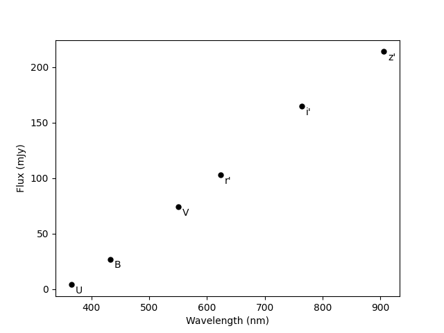
def plot_sed(multi_wl_fluxes):
"""Plot the spectral flux density in UBVr'i'z' in dependence of the
filter wavelength.
"""
wls = np.array([365, 433, 550, 623, 764, 906])
filters = ["U", "B", "V", "r'", "i'", "z'"]
plt.plot(wls, multi_wl_fluxes, 'ko', markersize=5.0)
for n in range(len(multi_wl_fluxes)):
plt.text(wls[n]+7, multi_wl_fluxes[n]-8, filters[n])
plt.xlabel('Wavelength (nm)')
plt.ylabel('Flux (mJy)')
plt.show()
return
def calc_abs_mag(mag, plx):
"""Calculate the absolute magnitude abs_mag from the relative magnitude mag
and the parallax plx in milli-second of arc.
"""
# Approximation of the distance dist in parsec:
dist = 1000./plx
abs_mag = mag - 5.*(np.log10(dist) - 1.)
return abs_mag
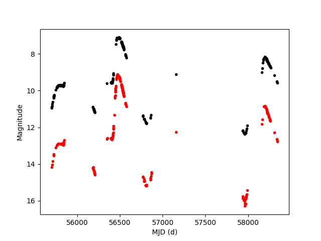
Light curves
The GDS contains light curves in up to 10 filters per observation field, among
which the r’ and i’ light curves contain the largest numbers of data points. We
can take a look at the r’ and i’ light curves of a star, e.g., the highly
variable V352 Nor:
r_mjds, r_mags = get_lc(241.71551, -52.07636, 1., "r")
i_mjds, i_mags = get_lc(241.71551, -52.07636, 1., "i")
plot_ts(r_mjds, r_mags, i_mjds, i_mags)
The result is:
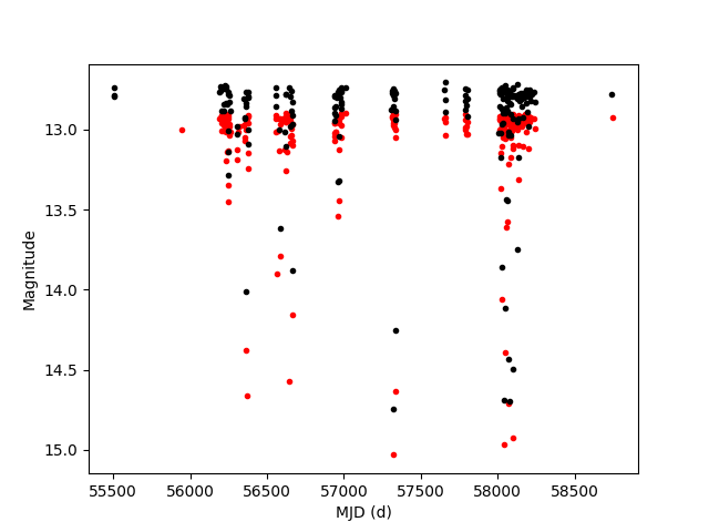
Period determination
The periods of many periodic variables in the GDS are still unknown or
uncertain. Short periods are not obvious when looking at the
(unfolded) light curve, as is the case for the eclipsing binary EH Mon:
r_mjds, r_mags = get_lc(103.03654, -7.06476, 1., "r")
i_mjds, i_mags = get_lc(103.03654, -7.06476, 1., "i")
plot_ts(r_mjds, r_mags, i_mjds, i_mags)
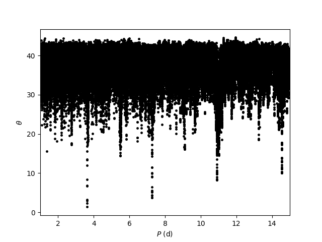
Among the numerous options for an automated period classification, here we
will use the Lafler-Kinman algorithm.
The light curve is folded by trial periods and the sum of squares θ of the
differences between two magnitude measurements of adjacent phase is calculated.
Basically, θ measures how smooth a folded light is when folded by a trial
period. Usually, θ is minimized when a light curve is folded by a multiple of
the correct period, therefore, test values with local minima in θ are the best
candidates for the period, in order from low to high.
r_p, r_p_candidates, r_theta_list = find_p(r_mjds, r_mags, 1., 15., 1e-4)
i_p, i_p_candidates, i_theta_list = find_p(i_mjds, i_mags, 1., 15., 1e-4)

# Exemplarily plot theta for the filter i':
plot_theta(i_p_candidates, i_theta_list)
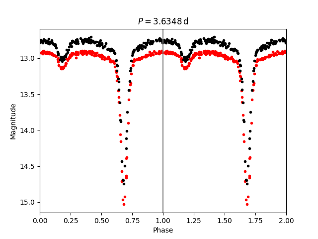
# The final period p is the average between period results from the
# r' and i' light curves:
p = (r_p + i_p) / 2.
plot_phase(r_mjds, r_mags, i_mjds, i_mags, p)
Multi-wavelength catalogue
Median magnitudes and light curves are not only available separately for
filters and fields, but there is also a multi-wavelength photometry catalogue
that is matched with Gaia DR3 sources. The filter magnitudes can be noticeably
effected by reddening; in this case, the roughly estimated spectral types from
the GDS UBV photometry might be more useful. For
Gaia DR3 5334136458661121280, median magnitudes in UBVr’i’z’ are available:
gdr3_id, multi_wl_mags, multi_wl_fluxes, spt = get_multi_wl_set(
    175.11591, -62.02608, 1.)
print("Gaia DR3 ID: " + gdr3_id + ", Spectral type from UBV photometry: " + spt)
print(f"U = {np.round(multi_wl_mags[0], 3)}, "
    f"B = {np.round(multi_wl_mags[1], 3)}, "
    f"V = {np.round(multi_wl_mags[2], 3)}, "
    f"r' = {np.round(multi_wl_mags[3], 3)}, "
    f"i' = {np.round(multi_wl_mags[4], 3)}, "
    f"z' = {np.round(multi_wl_mags[5], 3)}")
plot_sed(multi_wl_fluxes)
The result is:
Gaia DR3 ID: 5334136458661121280, Spectral type from UBV photometry: K5
U = 14.15, B = 12.996, V = 11.781, r' = 11.366, i' = 10.853, z' = 10.551
The match with Gaia DR3 allows to directly get information from the
Gaia DR 3 catalogue like the Gaia DR parallaxes to compute absolute
magnitudes:
gdr3_set = service.search(
    "SELECT parallax FROM gaia.dr3lite WHERE source_id=" + gdr3_id)
plx = gaia_set.getcolumn("parallax")[0]
multi_wl_abs_mags = np.zeros(6)

for n in range(len(multi_wl_abs_mags)):
    multi_wl_abs_mags[n] = calc_abs_mag(multi_wl_mags[n], plx)

print(f"M_U = {np.round(multi_wl_abs_mags[0], 3)}, "
    f"M_B = {np.round(multi_wl_abs_mags[1], 3)}, "
    f"M_V = {np.round(multi_wl_abs_mags[2], 3)}, "
    f"M_r' = {np.round(multi_wl_abs_mags[3], 3)}, "
    f"M_i' = {np.round(multi_wl_abs_mags[4], 3)}, "
    f"M_z' = {np.round(multi_wl_abs_mags[5], 3)}")
This gives:
M_U = 10.193, M_B = 9.039, M_V = 7.824, M_r' = 7.409, M_i' = 6.896, M_z' = 6.594
Columns
Sorted by DB column index. [Sort alphabetically]
| Name | Table Head |
Description | Unit | UCD |
|---|
| obs_id |
Obs_id |
Main identifier of this observation (a single object may have multiple observations in different bands and fields)
|
N/A |
meta.id;meta.main |
| ra |
Ra |
ICRS right ascension for this object as mean of the positions obtained from source extraction.
|
N/A |
pos.eq.ra;meta.main |
| dec |
Dec |
ICRS declination for this object as mean of the positions obtained from the source extraction.
|
N/A |
pos.eq.dec;meta.main |
| med_mag_nb |
〈mag〉 |
Mean magnitude in Astrodon NB.
|
mag |
phot.mag;em.line;stat.median |
| err_mag_nb |
Err〈mag〉 |
Error in median magnitude in Astrodon NB
|
mag |
stat.error;phot.mag;em.line |
| amp |
Amplitude |
Difference between brightest and weakest observation.
|
mag |
phot.mag;em.line;arith.diff |
| flux |
〈flux〉 |
Median flux in the Astrodon NB band; this is computed from the median magnitude based on Landolt standard stars.
|
mJy |
phot.flux;em.line;stat.median |
| err_flux |
Err〈flux〉 |
Error in median flux in the Astrodon NB band
|
mJy |
stat.error;phot.flux;em.line |
| nobs |
#Obs |
Number of observations of this object
|
N/A |
meta.number;obs |
| field |
Field |
Survey field observed.
|
N/A |
meta.id;obs.field |
| gdr3_id |
GDR3 |
Gaia DR3 source_id of this object.
|
N/A |
meta.id.cross |
Columns that are parts of indices are marked
like this.
Other
The following services may use the data contained in this
table:
VOResource
VO nerds may sometimes need
VOResource XML for this table.