Table information for 'rome.raw_series'

General

Table Description: Time series observed with ROME/REA in a custom scheme.

This table is not available for ADQL queries and through the TAP endpoint.

Resource Description: The ROME/REA (Robotic Observations of Microlensing Events/Reactive Event Assessment) Survey was a Key Project at Las Cumbres Observatory (hereafter LCO) which continuously monitored 20 selected fields (3.76 sq.deg.) in the Galactic Bulge throughout their seasonal visibility window over a three-year period, between March 2017 and March 2020. Observations were made in three optical passbands (SDSS g', r', i'), and LCO's multi-site telescope network enabled the survey to achieve a typical cadence of ~10hrs in i' and ~15hrs in g' and r'. In addition, intervals of higher cadence (<1hr) data were obtained during monitoring of key microlensing events within the fields. This catalog includes the full timeseries photometry for all ~8 million stars, down to a limiting magnitude of i~18mag.

For a list of all services and tables belonging to this table's resource, see Information on resource 'ROME/REA Timeseries Photometry Data Release 1'

Resource Reference URL: Resource info

Citing this table

@MISC{vo:rome_raw_series,
  year=2024,
  title={{ROME}/{REA} Timeseries Photometry Data Release 1},
  author={Street, R.A. and Bachelet, E. and Tsapras, Y. and Hundertmark, M.P.G. and Bozza, V. and Bramich, D.M. and Cassan, A. and Dominik, M. and Figuera Jaimes, R. and Horne, K. and Mao, S. and Saha, A. and Wambsganss, J. and Zang, W.},
  url={http://dc.g-vo.org/tableinfo/rome.raw_series},
  howpublished={{VO} resource provided by the {GAVO} Data Center}
}

Copyright, License, Acknowledgements

• The ROME/REA data is licensed under the Creative Commons Attribution Share-Alike 4.0 License

  
• https://spdx.org/licenses/CC-BY-SA-4.0.html

• This data release is a public product of the ROME/REA Key Project survey conducted on the robotic telescope network of the Las Cumbres Observatory (LCO). Individual images used in the data reduction are freely available for download on the LCO archive (https://archive.lco.global/).

  It is important to clarify that the light curves available through this data release are not optimized photometric reductions of individual objects. Researchers intending to utilize this data set for publications are kindly requested to acknowledge this source by citing the present paper (Street et al 2024 2024PASP..136f4501S) along with the original work by Tsapras et al 2019 2019PASP..131l4401T.

  For research work that requires enhanced photometry for specific targets within this catalog, we encourage reaching out to us directly. Collaboration opportunities are sincerely welcomed, and we look forward to supporting further inquiries and investigations.

Resource Documentation

As a short example for how to explore this data using VO protocols, try this:

• Open TOPCAT and it's VO/TAP window. Select "GAVO DC TAP" from the server selection and hit "use service".

• We would like to find "unusual" time series; perhaps ones with a large range. To get a feeling for what "unusual" might mean, just fetch a few metadata rows like with a TAP query like this:

  SELECT TOP 7000 * FROM rome.time_series
  WHERE np_i>100 AND np_g>100
  

• Do a plane plot of that data, and ask TOPCAT to plot mag_i_max-mag_i_min against mag_g_max-mag_g_min.

• When you open a table view, you can inspect the metadata for the time series when clicking on a point in the plot.

• Let's inspect the actual data: In TOPCAT's main window, do Views/Activation Actions. If you check "Plot Table", TOPCAT will download and plot the time series; it will only plot the first lightcurve, though. To get all bands, at this point you have to manually fetch accref from the table and use File -> Load Table. Sorry about this.

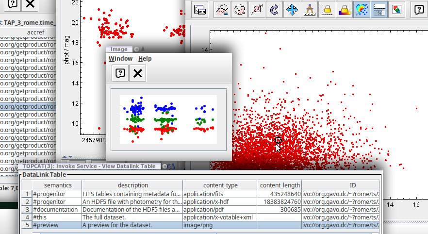
• Using datalink, you can also view three-band previews with one click on a plot point. To configure this, check "Invoke Service" in the Activation Actions, then use "Invoke now". In the dialog that pops up then, select the row with #preview and check Auto-Invoke. You will then see a light rendition of the light curves in (up to) three colours.

Your desktop could then look somewhat like this:

Columns

Sorted by DB column index. [Sort alphabetically]

Columns that are parts of indices are marked like this.

VOResource

VO nerds may sometimes need VOResource XML for this table.